Double the Context — What Becomes Four Times as Much?

In one line

The computation of one transformer layer splits into two shares. The scoring and mixing of attention grow with the square of the context length, and the remaining linear transformations grow in proportion to the length. At short contexts the latter dominates, and beyond a certain length the former dominates — knowing where that point is is the whole of this text.

Why this was needed

Every team gets a request to extend the context limit. From 4 thousand to 8 thousand, from 8 thousand to 32 thousand. When asked how much more expensive it gets, people answer "about double" and are then surprised when they see the bill, again and again.

The reverse also happens. You doubled the context and the cost only doubled, so you say "I thought it was quadratic, but no" and move on. Both come from the same misunderstanding. You are looking at only one side.

Two computations of different character are mixed inside one layer. Attention sweeps the whole context at every position, so as the number of positions grows, the sweeping grows with it and becomes a square. On the other hand, the projections that make the query, key and value, the output projection and the feed-forward are work that runs once for each position in the same way, so they are proportional only to the number of positions.

So the statement "quadratic in context length" is only half right. Precisely, it is the sum of a share that grows as a square and a share that grows in proportion, and which side dominates is decided by the length and the model width together.

What to count

You must not measure time here. The same code differs with the machine and the load, and inside a container it wobbles even more. Instead you count the number of multiplications. The count is the same integer wherever you run it.

How to count is simple. The dot product of two vectors of length d is exactly d multiplications. For the rest, you only need to count how many dot products go in.

def dot(a, b, ctr):
    total = 0.0
    for x, y in zip(a, b):
        total += x * y
    ctr.add(len(a))      # 곱셈 d 번을 장부에 적는다
    return total

If you measure the definition of attention with this yardstick, it comes out like this.

• Score matrix QK: n rows and n columns, and each cell is a dot product of length d → n * n * d
• Mixing AV: what comes out is small, n x d, but each position sweeps the whole context of n entries → again n * n * d
• Even if you split into h heads, the sum is the same. Each head's width shrinks to d / h, and there are h such heads.

So the share that grows as a square is 2 * n * n * d. For the other side, you count the cost one position pays just once and multiply by the number of positions.

• The three projections for query, key and value and one output projection → 4 * d * d per position
• Two feed-forward layers → 2 * d * d_ff per position

Together that is 4 * d * d + 2 * d * d_ff per position, and there are n positions.

The crossover point

If you put the two formulas side by side, the crossover point can be solved by hand. You find the smallest n for which 2 * n * n * d is at least n * (4 * d * d + 2 * d * d_ff). Dividing both sides by 2 * n * d reduces the condition to n >= 2 * d + d_ff.

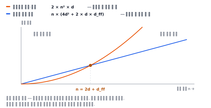
The feel that the numbers give is what matters. The wider the model, the more the crossover point shifts back. The linear cost one position pays grows with the square of the width, whereas the attention side grows only in proportion to the width. The impression in large models of "they said quadratic, so why don't I feel it" comes from here — you are still before the crossover point.

And once you pass the crossover point, the story changes. If you double the length, the total starts to approach four times.

The half that the causal mask throws away

A decoder's attention has a causal mask. The i-th position looks only up to itself, so the row length grows 1, 2, 3 and ends at n. The scores actually used number n * (n + 1) / 2.

The matrix is still n squared cells. So nearly half is computed and thrown away. To be exact, (n - 1) / (2 * n) is thrown away, and as the length grows it approaches half.

An implementation that naively computes everything and then covers it with a mask does exactly that. To reduce the computation, you must not apply the mask afterward but not compute those entries at all, and that is how kernels that run only the triangle in block units appeared. It is the same reason that PyTorch's scaled_dot_product_attention takes is_causal separately. Receiving the mask as a tensor and multiplying, and telling it "this is causal", do different work inside.

Memory has the same shape

If you hold the score matrix whole, the number of values is n squared per head. In total it is n * n * h, and multiplying by the bytes of one element of the data type gives the bytes.

You can tell why this hurts by turning it around. If you fix a budget and find the maximum length that fits, you must quadruple the budget to double the length. It means that even if you double the number of cards, you can extend the context only 1.41 times.

That is why implementations that do not build the whole score matrix became important. If you cut it into blocks, process one piece at a time and discard it, you do the same computation while holding fewer values. The amount of computation stays the same and only the memory shrinks — without a sense that these two move independently, you cannot understand "why does a longer context become possible when the computation is the same".

The length you feed in and the length you produce grow differently

Feeding in a prompt all at once (prefill) and producing tokens one at a time (decode) grow in different shapes.

Prefill processes n positions at once, so the scores arise on the scale of n squared. On the other hand, if you attach one more after n have already piled up, the one new query just looks at n + 1 keys. It is one row. So the total of the scores produced while making g tokens is g * n + g * (g + 1) / 2.

An interesting identity comes out here. If you set n to 0, this value is exactly equal to causal_pairs(g). Whether you feed it in at once and erase with a mask or attach one at a time, the number of scores actually needed is the same. All that differs is whether you do it at once or in pieces. What makes up for that difference is the subject that the KV cache documentation deals with, and it is the job of the next module.

What it looks like in the field

First, you doubled the context limit, latency did not double, and you feel reassured. You are still before the crossover point, so the linear share is just dominating. If you extend the length further, the slope suddenly changes.

Second, the same length, but the shape of the cost curve changes when you switch models. If the width differs, the crossover point is in a different place. If you use a ratio measured on one model as it is on another, it goes off.

Third, memory blows up first at long contexts. The computation holds, but there is no room to hold the score matrix. Even if computation and memory are the same n squared, the wall that you hit first is usually memory.

Fourth, an implementation that builds the mask as a tensor and multiplies is twice as slow. It is because it computes everything and throws half away. Even with the same formula, the actual amount of work splits on when you apply the mask.

Fifth, prefill is slow but token generation is fast. Or the reverse. The two grow in different shapes, so if you make an estimate by lumping them into one ratio, one side is sure to be wrong.

What really matters in practice

• Do not just memorize the word "quadratic"; split it into two shares. Which side dominates is decided by length and width together.
• Count the number of operations instead of time. The count is the same even when the machine changes, and it is the basis when you explain an estimate to others.
• Work out the crossover point with your own model's numbers. Capacity planning differs before and after that point.
• Look at computation and memory separately. Even with the same n squared, the ways to reduce them differ.
• Measure prefill and decode separately. A single ratio is sure to make one side wrong.

What you will do in the next lab

You grow /root/work/tf-cost/cost.py one step at a time. You use only the standard library — the system Python of this Pod has no numpy (it exists only inside /opt/onnx-lab/bin/python) and no torch or transformers either. Instead you build by hand a counter that counts multiplications and use only the integers that come out of it.

You start with the counter and the dot product, then actually run the score matrix and the mixing and confirm by counting that n squared comes out. Next you actually run the six linear transformations that one position pays, confirm that this side is independent of length, and build a table that puts the two shares side by side.

From that table you find the crossover point. You also see, with your own numbers, where the crossover point moves as you vary the model width. Then you count the scores that the causal mask leaves, confirm that half are thrown away, and work out the bytes when holding the whole score matrix and the maximum length that fits within a budget.

The last step is the point of this lab. You count that attaching one token produces only one new row of scores, and you confirm with integers the identity that the total when producing g tokens from length 0 is exactly equal to the number the causal mask leaves. The grader actually imports your module, pokes at the functions with different sizes every time, and even checks how far the counter actually went up. You cannot memorize values and plug them in.