
I sent 3.3 V. Why did 5.5 V arrive?
In one line
A cable is not a teleportation device. A fast voltage change travels along the line, and if the impedances at the two ends differ, it comes back. A received voltage larger than the voltage you sent can also be the result of this reflection.
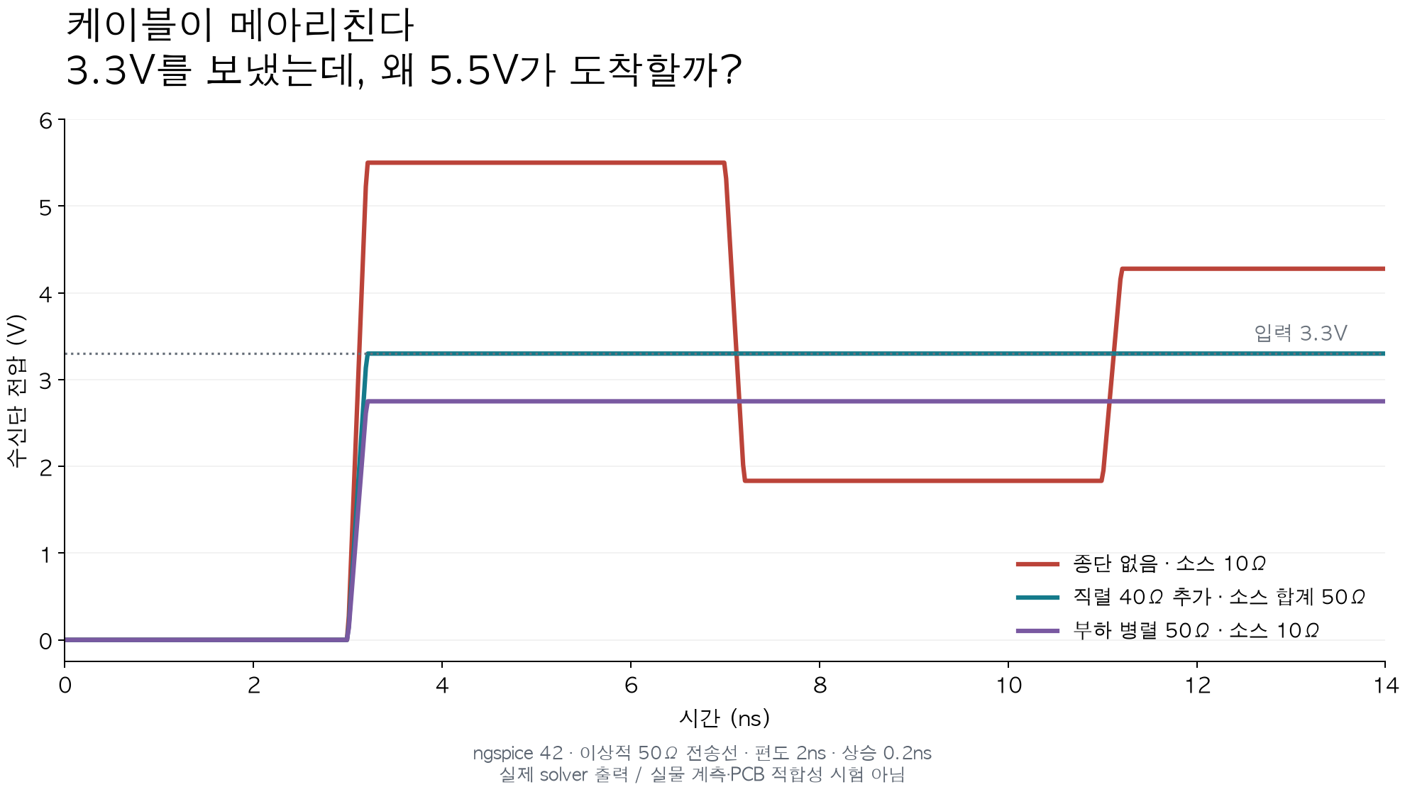
The figure is real solver output calculated under the same nominal conditions as this course. It is not a physical measurement. Read the legend and the voltage and time axes along with the colors of the lines.
Why this was needed
"I set the output to 3.3V, but 5.5V shows up at the input." Your first reaction would probably be to suspect that the instrument is broken. But when the forward wave and the reflected wave add at the boundary of a transmission line, an instantaneous voltage higher than the supply voltage can arise. In this lesson we reproduce that phenomenon with ngspice's ideal transmission line model, without connecting any equipment. It does not mean you have checked the allowed voltage of a real board.
In a slow circuit, treating the line as a single uniform potential does not readily reveal problems. But if the rise time of the signal is short compared with the propagation time, the receiving end is still in its old state while the transmitting end changes. The important comparison is not simply how many times per second data is sent but how fast the edge changes. Even a signal sent infrequently may need this review if its edge is fast.
If you learned resistive dividers in an earlier introduction to electronic circuits, the starting point is the same. What changes is what the transmitter sees at first. Before a wave has traveled to the load and back, it cannot know immediately that the far-end resistance has changed. First it divides the voltage with the line's characteristic impedance Z0, and later the returning wave changes the state of the transmitting end.
How it works
Let's first fix the names and units of this model. Vs is the supply voltage in V, Rs is the driver plus the added series resistance in Ω, Z0 is the line's characteristic impedance in Ω, and RL is the load resistance in Ω. TD is the one-way propagation time. Instead of entering the physical length of the line directly, you specify Z0 and TD, which in effect summarizes the dielectric and the wiring structure in these two numbers.
| Item | Reference condition | Meaning |
|---|---|---|
| Supply | 3.3V, begins rising at 1ns | Not a signal that turns on at time 0 |
| Edge | Rise time 0.2ns | A short slope, not an ideal vertical line |
| Source | Driver 10Ω, added 0Ω | Total Rs is 10Ω |
| Line | Z0=50Ω, TD=2ns | The round trip takes 4ns |
| Load | 1GΩ | Very large but not infinite |
The magnitude A of the voltage that first goes forward is found by voltage division. The reflection coefficient shows how different the boundary's resistance is from the line, and it has no unit. The wave reflected at the load is A multiplied by ΓL. The voltage seen at the receiving end is the sum of the two waves, A×(1+ΓL).
A  = Vs × Z0 / (Rs + Z0)
ΓL = (RL - Z0) / (RL + Z0)
ΓS = (Rs - Z0) / (Rs + Z0)
첫 수신 평탄부 = A × (1 + ΓL)
두 번째 수신 평탄부 = A × (1 + ΓL) × (1 + ΓS × ΓL)
Under the reference conditions, A is 2.75V. If the load is very large, ΓL is close to 1 and the first received plateau is about 5.5V. The driver's 10Ω is smaller than the line's 50Ω, so ΓS is negative. When the returning wave is reflected at the source and arrives at the load again, the next change is in the negative direction. Rather than "reflection always makes it bigger", you must look at the sign of the reflection coefficient and the accumulated waves together.
Count the times too. The transmit edge departs at 1ns, so the receive edge appears from 3ns. You can read the first plateau only after the 0.2ns rise time has passed. The wave returning from the load reaches the source around 5ns, and the wave sent out again from there reaches the load around 7ns. If you mistake TD for the round-trip time and enter 4ns, the voltage may look plausible but the order of events changes.
The CSV's time_s is in seconds, and the time fields of the input JSON are in ns. The same time appears as 3e-9 in the CSV and as 3ns in the explanation. When you find the threshold-voltage arrival time, you find the two samples that bracket the first threshold and interpolate along a straight line. If it is at or above the threshold from the first sample, return the first time, and if it never reaches it by the end, return None. If you unconditionally return 0, "it did not reach" and "it was high from the start" get mixed.
If you pick only the first point among the samples that is larger than the threshold, you record late even though the real crossing was earlier. For example, if it is 1V at 2ns and 3V at 4ns, the 2V crossing is 3ns by linear interpolation. This calculation is a numerical convention that approximates the interval between two points as linear. It is not the result of measuring every detail of the real electromagnetic field.
What it looks like in the field
Signal integrity work is not looking at a single output number. You must build the circuit and wiring model, interpret the time and voltage of the waveform, and explain why the ideal prediction and the real measurement differ. We carried the transmission line theory, simulation, and scripting requirements from a public NVIDIA SI/PI role posting into this activity. One posting does not guarantee the whole hiring market or your employability.
In real hardware, loss, input capacitance, packages, connectors, vias, and the measurement probe are added. The ngspice T element here is an ideal single-mode lossless line. To select real cable materials or to judge that a PCB meets its ratings, additional models and measurements are needed. The role of this course is to first isolate and learn the principle in a limited model.
What to learn next
In the next module you see why one resistor changes the reflection. In the lab of the last module, you read the CSV the real solver made and calculate the arrival time and reflected voltage with Python functions. Instead of simply copying the example numbers, you satisfy the same contract under other voltage and resistance conditions.