Calibration Data Builds the Ruler: Too Narrow Clips, Too Wide Blurs

In one line

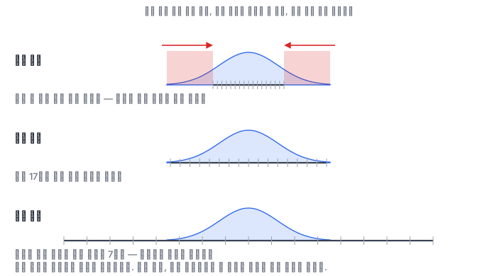
In static quantization, the scale is decided by the calibration data. If the range the calibration saw is narrower than the real distribution, values get clipped, and if it is wider, the grid gets coarse — either way, accuracy is a function of the calibration data.

Why it keeps collapsing here

Static quantization pins down the scale of the activations at conversion time. To pin it down you have to know what range the activations live in, and the calibration data is what tells you that. The converter feeds this data through, observes the minimum and maximum of each layer, and makes the scale and zero point from that range.

So calibration data is an input value, not a setting. With the same model and the same conversion command, changing only the calibration data gives a completely different model. Yet this data is not left in the code and is not in the logs either. A few months later, when someone asks "why is this model's accuracy like this", there are only the model file and the conversion script, and what actually decided the answer was the arrays used that day.

There are two directions of collapse. If it is narrow, it gets clipped. When a value larger than the maximum seen during calibration comes in, it sticks to the end of the integer data type and does not come back with dequantization. The error grows to tens of times the round-trip upper bound. If it is wide, it gets squashed. It distributes the 256 grid steps over a wide range that is not actually used, so only a few grid steps lie in the interval where the data actually lives. It is not clipped, but it loses resolution.

A figure setting the calibration range over the same activation distribution in three ways: narrow, right and wide. If narrow, both ends are clipped and values outside the range stick to the integer ends; if right, the grid lies evenly over the data; if wide, only a few grid steps lie in the interval where the data lives, losing resolution

How it works

The ONNX Runtime quantization documentation says to pass a CalibrationDataReader to static quantization. The contract is short.

class 내_공급기(CalibrationDataReader):
    def get_next(self):
        더 줄 것이 있으면 -> {"입력이름": 배열}  사전 하나
        더 없으면        -> None

The converter keeps calling get_next() until None comes out. So two mistakes are common. One is throwing an exception instead of None after it ends (it dies in the middle of calibration), and the other is reusing a provider that has already been exhausted (the second conversion receives no calibration data at all).

The trace calibration left is right there inside the model. If you open the graph, find the QuantizeLinear right after the input and read its scale initializer, the scale times the number of grid steps is the width of the range observed during calibration. With this one number, you can check after the fact "how far the calibration data saw".

There are two formats too. QDQ leaves the original operator as it is and inserts QuantizeLinear and DequantizeLinear before and after. MatMul is still visible in the graph, and the runtime fuses the integerization at execution time. QOperator swaps it out entirely for an integer operator such as QLinearMatMul. The node count is small and the file is small too, but the graph is hard to read.

One common misunderstanding must be pointed out here. Two formats extracted from the same calibration use the same scale and zero point and have errors of the same order of magnitude, but they are not identical element by element. That is because QDQ leaves the original operator in the graph and leaves the way of executing to the runtime. The runtime may fold the Q/DQ and run an integer kernel, or it may just do real-number arithmetic on the dequantized values. So "I switched the format and the output changed slightly" is normal, and if the order of magnitude changed, then you must suspect the calibration.

What it looks like in the field

First, there is a kind that does not get fixed even if you increase the samples. If the distribution of the calibration data itself is off, even increasing that data hundreds of times widens the observed range only a little. The improvement from increasing a narrow calibration 512 times is worse than giving just a few batches from the right distribution. You have to tell by measuring that sometimes it is the distribution, not the count, that is the problem.

Second, static is not always more accurate than dynamic. "Static is better" is a statement about when calibration is done properly. If the calibration is off, you get a model much worse than dynamic quantization. And that fact does not show up anywhere until you evaluate.

Third, clipping and squashing have different symptoms. Clipping errs greatly only on large inputs and is fine on small ones. Squashing errs a little evenly on all inputs. If you split the error by input size, you can tell which it is.

Fourth, keep the calibration data as a record. Write next to the model which samples you used and how many, and what the range of that data was. You can find the cause later only if you can cross-check it against the scales inside the model.

What really matters in practice

Draw the calibration data from the same distribution as the data that will come in at deployment. This comes before the number of samples.
Take out the scales pinned in the model and check them. The scale times the number of grid steps is the range the calibration saw.
Measure with three sets. If you quantize three times — narrow, right and wide — you see the sensitivity of your own data.
The format is a difference of representation, and the runtime decides the execution. If changing the format changes the error by an order of magnitude, suspect the calibration.

What you will do in the next lab

You implement a CalibrationDataReader yourself, quantize the same model with three sets of calibration data — narrow, right and wide — and write side by side the input scale pinned in the graph and the maximum absolute error you measured. Then you grow the narrow calibration from 1 batch to 512 batches to measure that it cannot be fixed that way, and finally you extract QDQ and QOperator from the same calibration and measure together the error magnitudes of the two formats and the difference between them. The grader drives your provider directly and recomputes the errors you wrote out with your model file to check against them.