Data skipping indexes and projections — speeding up filters outside the sort key

In one line

A skipping index is not a B-tree pointing to row positions but a summary attached to each bundle of granules (minimum and maximum, a set of values, a Bloom filter), and it skips that bundle only when it can say "it is definitely not here". A projection is another sorted (or pre-aggregated) copy hidden inside the part. Both must be MATERIALIZEd to exist in parts that are already there, and both pay with disk.

Why this was needed

In the earlier modules we saw that the sorting key decides almost everything. But there is only one sorting key. If you sort a log table by time (ts), "yesterday afternoon" is fast, but when you look for "this one trace_id line" in an incident investigation, it reads all 1 million rows. In a row-oriented database you would build one more secondary B-tree index. The official documentation explains that this approach does not work in column-oriented storage — because there is no separate "row" on disk to point to.

ClickHouse's answer goes two ways. One is finding out more granules that do not need to be read (skipping indexes), and the other is keeping one more copy with a different sorting key (projections, or the materialized views of the earlier module). Which is right is decided by the distribution of the data.

How it works

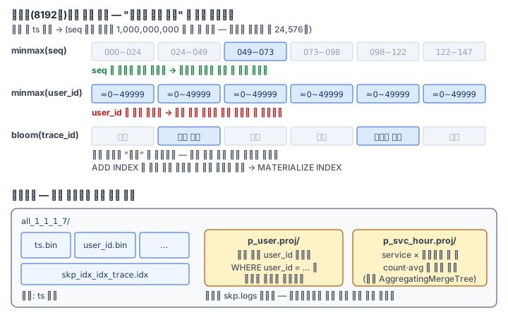
An index is defined by four things — a name, an expression, a kind (TYPE) and GRANULARITY. GRANULARITY is how many granules to summarize as one bundle. With 1 it is one summary per 8192 rows, and with 4 one per 32768 rows. The kinds introduced in the documentation are these.

Kind	What it records per bundle	Good fit
minmax	Minimum and maximum of the expression	Range conditions on a column that grows roughly along with the sorting key
set(N)	Up to N distinct values (empty if exceeded)	A column that is varied overall but has only a few values within a bundle
bloom_filter	A Bloom filter of the set of values (false-positive rate default 0.025)	Finding one rare value, "a needle in a haystack"
ngrambf_v1, tokenbf_v1	A Bloom filter of n-grams or tokens	Partial string search — deprecated from 26.2, the text index is recommended

On this Pod (26.8), when you run ADD INDEX idx_trace trace_id TYPE bloom_filter GRANULARITY 1 on a table with 1 million rows and 123 granules, a Skip slot appears in EXPLAIN indexes = 1 but it is Granules: 123/123. Only the definition was created, and existing parts have no index file (a size of 0 in system.data_skipping_indices). As the documentation says, it applies only to newly arriving data. ALTER TABLE ... MATERIALIZE INDEX idx_trace is a mutation that creates the files in existing parts, so the part name changes from all_1_1_1 to all_1_1_1_2, and after that it is Granules: 3/123, with 24,576 rows read. The row you are looking for is one line, but because of the Bloom filter's false positives it read two more granules.

Even with the same minmax, the results are at opposite extremes. A range condition on seq, which grows with time, left only 1/123 granules, while user_id, evenly spread regardless of time, has values near the minimum and near the maximum in every granule, so it was 123/123, that is, it skipped not one. As the documentation puts it, a useful skipping index usually requires a strong correlation between the sorting key and the target column. Even if a value is in a bundle only once, the whole bundle has to be read, so without correlation the index only adds computational cost.

In that case, what you use is a projection. After ADD PROJECTION p_user (SELECT * ORDER BY user_id) and MATERIALIZE PROJECTION, a copy re-sorted by user_id is created for each part. The query still points at skp.logs, and the optimizer picks the side with the least to read. On this Pod, WHERE user_id = 4242 dropped from 1 million rows to 8,192 rows, and skp.logs.p_user was left in the projections column of system.query_log. A projection with a GROUP BY becomes a hidden AggregatingMergeTree and thus a pre-aggregated copy. The count and avg projection per service and hour was 4,320 rows, and the per-service aggregation query read only that instead of the original.

The price is paid in disk. On this Pod the p_user copy was about 24.6MB, nearly half of the whole part including the copy (about 52.9MB). The aggregate projection was about 36KB, the Bloom filter index about 1MB, and the minmax index a little over 1KB. Projections have restrictions too — as the documentation says, you cannot give a TTL different from the original, you cannot chain them, you cannot use WHERE or JOIN in the definition, and if you run a lightweight DELETE on a table with a projection, it is rejected under the default setting (lightweight_mutation_projection_mode = throw) (error code 344 confirmed on the Pod).

Finally, one pitfall when measuring. The query condition cache (use_query_condition_cache), which is on by default in this Pod's 26.8, remembers "granules that had no rows matching this condition". When I ran a query with the same condition a second time, the rows read dropped from 1 million to 0. When comparing index effects, give use_query_condition_cache = 0 and measure.

What it looks like in the field

The most common mistake is, thinking "it's a column we often filter by, so let's put an index on it", to put a minmax or set on an evenly spread column. If the Skip slot of EXPLAIN is 123/123, that index has only cost. Before you add one, first see whether the target column is correlated with the sorting key.

The second is doing only ADD INDEX on a big table in production and wondering "why isn't it faster?". It is created only in new parts, so existing data has to be MATERIALIZEd, and that is a mutation that rewrites all parts — do it in quiet hours, watching progress with system.mutations.

The third is lookups of unique values such as trace_id and request_id. It is almost the only place where a Bloom filter fits well, and for partial string search, in 26.x you look at the text index first. You use a projection after you have judged that "a second sorting key is absolutely needed and doubling the disk is acceptable".

What you will do in the next lab

You insert 1 million rows into skp.logs and merge into one part. You save the EXPLAIN in the state where the Bloom filter index has only been ADDed, and measure the rows read after MATERIALIZE. You compare the effect by attaching minmax to seq and user_id, create a user_id projection and a service-and-hour aggregate projection and check them with query_log, and finally read from the system tables the disk all of these used.