What Storing by Column Means — Parts, Column Files, Compression

In one line

ClickHouse's MergeTree stores rows as a bundle of files (a part) that are sorted in sorting-key order and compressed separately per column. So the cost of a query is decided not by how many rows it selects but by which columns it touches and how much it can skip using the sorting key.

Why this was needed

If you throw analytic queries at a row-oriented database, you soon meet the question "why does it read the whole table just to get one sales total?" Row-oriented storage keeps all the columns of a row together, so even if you only want to add up the amount column, the disk fetches whole rows. For transaction processing that is right — you read and write a whole order at a time. But analytics is the opposite. You read two or three columns out of hundreds of millions of rows.

Column-oriented storage flips this asymmetry. If you gather the values of the same column together, a query only has to read the columns it uses, and because similar values sit next to each other, compression also works much better. In exchange, "changing a single row" becomes expensive, because several column files have to be touched. Most of ClickHouse's design decisions — a part, once written, is not modified; deletes and updates are handled later at merge time — come from this trade-off.

How it works

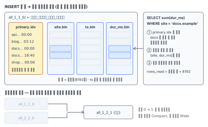
The four steps of an INSERT written in the official documentation (Table parts) are the storage structure itself.

1. Sort the incoming rows in the order of the table's sorting key (ORDER BY) and build a sparse primary index
2. Split the sorted rows into columns
3. Compress each column
4. Write the compressed column files and the index into one new part directory

Once a part is written it does not change (immutable). Each INSERT adds one more part, and background merges combine small parts into larger ones. The old parts that were combined become inactive and are then deleted. In the part name all_1_2_1, all is the partition, 1–2 is the first and last block numbers it contains, and 1 is the merge level. Level 0 is a part that has never been merged.

Inside a column file, the data is divided into granules. By default, 8192 rows make one granule, which is the smallest unit of processing. The primary index writes not every row but only one key value, the first row's, per granule — that is why it is a "sparse" index. When WHERE site = 'docs.example' arrives, it scans the index and skips, whole, the granules that cannot hold that value. If you filter by a column that is not in the sorting key, there is no basis to skip anything, so it reads everything. The marks in system.parts is the number of position markers attached one per granule, plus one more mark that signals the end (2 million rows give 245 granules and 246 marks).

Compression ratio varies a lot by column. A column in which the same value continues for a long stretch (the first column of the sorting key, a column with only a few distinct values) shrinks by hundreds of times, while near-random integers barely shrink. LowCardinality(String) is a type that stores strings by replacing them with dictionary numbers, so a column with five site names becomes almost free. Conversely, an integer that keeps growing, like a timestamp, does not shrink with the default codec (LZ4) alone — codecs that shrink it are covered in a later module.

SELECT name, data_compressed_bytes, data_uncompressed_bytes
FROM system.columns WHERE database = 'col' AND table = 'events';   -- 열별 크기

SELECT sum(dur_ms) FROM col.events FORMAT JSON;   -- 맨 끝 statistics 에 rows_read · bytes_read

There are two scales for measuring cost. rows_read is the number of rows read without being skipped, and bytes_read is the (decompressed) bytes of the columns touched in those rows. Summing one UInt32 column is 4 bytes per row, and for 2 million rows exactly 8,000,000 bytes. Even for the same 2 million rows, if you read the contents of a long string column it becomes several times that. There is one pitfall — length(url) is rewritten to read only the subcolumn (url.size) that holds the length, not the string contents, so it reads only 8 bytes per row. Do not guess what was read; confirm it with numbers.

These numbers for every query are also left in system.query_log. If you attach a tag with SETTINGS log_comment = '...', it is easy to find your own query later. The log table is flushed about once a second, so to see a query you just ran right away, first run SYSTEM FLUSH LOGS.

Finally, the format of a part. If the part is small, it becomes Compact, which puts all columns in one file, and if it is large, it becomes Wide, which keeps a separate file per column. The boundary is set by the table settings min_bytes_for_wide_part and min_rows_for_wide_part. It is a device to keep the number of files from exploding when small INSERTs are frequent.

What it looks like in the field

When you get a report that an analytics dashboard is slow, the first thing you look for is SELECT *. A habit that was almost free in a row-oriented database becomes the work of opening every column file in column-oriented storage. Often, merely changing it to select only the columns the screen needs cuts the bytes read to a fraction.

The second most common is a table whose sorting key was set to "it's the primary key, so id". If nearly every query filters by site and period and the sorting key is id, there is an index but it never skips anything. If rows_read is always equal to the total row count, suspect the sorting key.

The third is capacity planning. If you plan "the raw log is 100GB a day, so the disk is 100GB × retention days", you will be badly wrong. Because the compression ratio differs from several times to hundreds of times per column, it is right to load a real day of data, measure the post-compression size in system.columns, and multiply from there.

What you will do in the next lab

You create the col.events table with the sorting key (site, ts), insert 2 million rows, merge the parts into one, and read the name, row count and mark count from system.parts. From the per-column compression ratios you find the column that shrank best and the one that shrank least, and compare the bytes_read of a query that reads one column with one that reads a long string column. You measure rows_read when filtering by the sorting key versus by a column outside the key, find your own query in query_log, and then create one more small table to check a Compact part.