A Correct Value Read Too Early Is Still Wrong

In one line

The range of the steady state and the time to reach that state are different items to verify.

Why this was needed

A sensor that worked well on one development board goes out of range on only some units after mass production. The number printed on a resistor is a nominal value, not the measured value of every part. On top of that, supply error overlaps. One nominal calculation being right does not mean the design margin is sufficient.

Just because you use several ±1% resistors, you cannot simply set the voltage error to ±1%. That is because the output voltage depends on the ratios of the resistors. If only the top of a divider grows, the output goes down, but if only the bottom grows, it goes up. An experiment that scales everything by the same ratio misses exactly this worst combination.

How it works

If the supply and the three resistors each have two end values, you calculate 16 combinations. In this circuit, which has only positive resistances, the output increases when the supply, the bottom resistor, and the load grow and decreases when the top resistor grows, so the minimum and maximum of the end values set the range. It is not a general law that looking only at the corners is always enough for nonlinear elements or complicated circuits. Also, since no uniform or normal distribution was given, you cannot calculate a defect rate from this range.

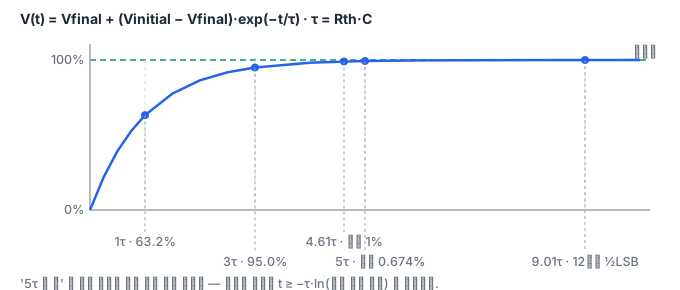
If you connect a capacitor C to the output, the voltage does not instantly become the final value. In an ideal first-order circuit, V(t)=Vfinal+(Vinitial-Vfinal)*exp(-t/τ). The time constant is τ=Rth*C. When you find Rth, you replace the independent ideal voltage source with 0 V, that is, a short. So in this circuit the top, bottom, and load resistors all look like they go to ground and are in parallel. If you set the supply resistance to infinity, you get a different time constant.

If the residual error relative to the final value must be 1% or less, exp(-t/τ)<=0.01, that is, t>=-τ*ln(0.01). Saying it has reached about 63.2% at 1τ is different from saying it has settled to 1%. Increasing C can make the change slower, but it conflicts with the time budget for reading the input quickly.

What it looks like in the field

The full sample interval of an ADC and the time for acquiring the input may not be the same. You must check the datasheet's acquisition time, the input circuit, and the allowed source resistance together. The 100 nF in this textbook is an educational capacitor added to the output and does not mean the internal sampling capacitor of a specific ADC. In practice you must also check the switch resistance, amplifier stability, and noise.

Bounds and probability are different questions

When the supply is highest, the top resistor is smallest, and the bottom and the load are largest, the output of this model is at its maximum. The opposite combination is the minimum. Counting all 16 combinations here does not mean measuring 16 production units. It lays out the possible boundaries. Just because a bad result appeared at an end value, you cannot say 1/16 of the product is defective. If you do not know the real distribution and the correlations between the variables, that ratio does not exist.

In practice, you record the "room-temperature nominal value", the "electrical tolerance range", the "temperature variation", and the "part aging" separately. This ±1% does not add a temperature coefficient or long-term drift. So even if the tolerance calculation passes, temperature verification is not finished. Lumping all unknown effects together and adding a casual 10% margin looks conservative, but you cannot explain what you missed and what the basis of that number is.

Check the waveform at three points

You can check an RC calculation with three points: the initial value, one time constant later, and a sufficiently long time later. In a separate example that goes from an initial 0 V to a final 2 V with τ=2 ms, it is 0 V at t=0, about 1.264 V at t=2 ms, and about 1.987 V at t=10 ms. If the voltage exceeds the final value or falls as time passes, you have written the exponent sign or the initial condition wrong. This monotonic rise is a property of this passive first-order charging model, and it is not generalized to cases with inductors or where oscillation arises in active circuits.

The expression "done at 5τ" must also be used together with the required error. The residual error after 5τ is about 0.674%. It is enough for a 1% criterion but may not be enough for a high-resolution converter that demands a much smaller error. At 12 bits, half an LSB of a full-scale step is 1/8192 of the full range, so even the ideal first-order model alone needs about ln(8192)=9.01τ. Whether the size of the real acquisition step is full scale, and the other error budgets, must be set separately.

The capacitor's 100 nF is 100×10⁻⁹ F. If you write it as 100e-9 in Python, you can unify the units before the calculation. If you want to show the time result in ms, finish the calculation in s and multiply by 1000 at output time. If you mix ms and s in the intermediate calculation, even a response that is wrong by a factor of a thousand is drawn as a smooth curve. A graph looking plausible and the units being right are different verifications.

Finally, the supply going to 0 V does not make the resistor disappear. Looking in from the output, the top resistor is also connected to ground, so it remains together with the other two resistors. Redrawing the circuit diagram once prevents this kind of error more reliably than memorizing one complicated formula.

Next check

The quiz that follows distinguishes tolerance combinations from time criteria. In the lab of the last module you build the 16 tolerance combinations and calculate how far the nominal circuit has reached after 1 ms. Instead of saying you used measurement equipment, describe the result as "a prediction of the ideal first-order model". Also examine the trade-off that a larger resistance reduces power consumption but may increase the output impedance.