A shuffle is the most expensive step, and 200 partitions is a number chosen without knowing your data

In one line

A shuffle is every partition sending data to every partition in order to gather the same key in one place, and it pays for disk writes, serialization and the network all at once. The number of partitions after a shuffle is 200 by default, a fixed number regardless of data size. AQE merges small partitions during execution, but you have to check for yourself what was merged and the difference between repartition and coalesce.

Why a shuffle is a problem

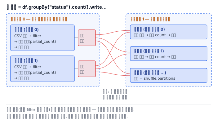
filter and withColumn take one partition and produce one partition. They do not need to look at neighboring partitions, so they finish inside a single task. These are called narrow transformations. groupBy, join, distinct and orderBy are different. You do not know in which partitions the same key is scattered, so to compute, you have to search all the partitions and gather the same keys together.

The shuffle section of the RDD guide calls this Spark's mechanism for redistributing data between partitions, and gives three reasons it is expensive: disk I/O, data serialization and network I/O. The side that prepares the shuffle is called the map tasks and the side that gathers and computes is called the reduce tasks; the documentation adds that these names come from MapReduce and are not directly related to Spark's map and reduce operations.

It works like this. A map-side task collects its results in memory, and when memory overflows, it sorts them by destination partition and writes them to a file. A reduce-side task reads, from the files written by all the map tasks, only the blocks that are its own share. The documentation says that a shuffle creates many intermediate files on disk and, in case the lineage has to be recomputed, keeps those files until the references disappear. So a long job with many shuffles eats a fair amount of disk.

How it works: the number 200

Someone has to decide how many partitions to divide into after a shuffle. For DataFrames and SQL, that value is spark.sql.shuffle.partitions in the performance tuning documentation: the number of partitions used when shuffling for joins or aggregations, with a default of 200.

200 is not a number chosen by looking at the data. For 1TB it is too few, so one partition comes to around 5GB, memory overflows and it spills to disk. For 300,000 rows it is too many: a few hundred rows go into each partition, and the fixed cost of launching and collecting 200 tasks is greater than the work. If you write that result straight to files, each write task writes a file, so small files pour out.

spark.conf.set("spark.sql.adaptive.enabled", "false")    # AQE 를 끄고 날것을 본다
by_day = orders.groupBy("day").agg(F.sum("qty"))
by_day.write.mode("overwrite").parquet("/root/spk/out/by_day")   # 셔플 뒤 태스크 200개
spark.conf.set("spark.sql.shuffle.partitions", "8")        # 자료에 맞춰 줄인다

AQE merging partitions

The reason it is hard to set the number by hand is that you do not know the size after the shuffle until you shuffle. The section on coalescing post-shuffle partitions solves this problem. When both AQE and spark.sql.adaptive.coalescePartitions.enabled are on (both default to true), it looks at the map-side output statistics and merges adjacent small shuffle partitions. If you do not give the initial number of partitions initialPartitionNum, it equals spark.sql.shuffle.partitions.

There are details in how far it merges. The default of the target size advisoryPartitionSizeInBytes is 64MB, but parallelismFirst defaults to true, so it ignores this target size, keeps only the minimum size minPartitionSize (default 1MB), and maximizes parallelism. The documentation recommends setting this to false on a busy cluster so that small tasks do not multiply. In other words, AQE with default settings does not "bundle up to 64MB". The merged result appears in the final plan as AQEShuffleRead ... coalesced.

repartition and coalesce

There are two ways to change the number of partitions directly, and their costs are completely different. repartition creates a new hash-partitioned DataFrame. It redistributes every row, so a shuffle occurs. In return, the partition sizes become even, and if you give columns, the same values gather in the same partition.

coalesce is a narrow dependency. In the documentation's example, reducing from 1000 to 100 makes each new partition take over 10 existing partitions without a shuffle. If you ask it to increase, it stays at the current number. On the other hand, the documentation warns that a drastic reduction such as coalesce(1) can make the computation itself run on fewer nodes. Because there is no shuffle, the preceding stages are merged into one task. In that case, even though it costs one shuffle, repartition lets the preceding stages run in parallel.

The RDD guide lists coalesce among the operations that can cause a shuffle, because the RDD coalesce takes whether to shuffle as an argument. The DataFrame coalesce has no shuffle, as explained above. In SQL, the partition hints COALESCE, REPARTITION and REBALANCE do the same job, and the documentation also introduces them as tools for reducing the number of output files.

What it looks like in the field

200 files from small data. A job run on development data fills the output folder with files of a few dozen bytes. One setting is enough to see the cause. If AQE is on, it shrinks a lot, but it is more reliable to fix the number of files with coalesce just before writing.

The shuffle volume is in the log and the UI. The Stages tab of the web UI shows Shuffle read and Shuffle write for each stage in bytes and records, and the task end events in the event log contain the same metrics. Instead of a feeling that "the shuffle is big", you speak in numbers.

A job with only narrow transformations has one stage. A job that only reads, filters and writes has no shuffle, so it has one stage. If there are two or more stages, it is evidence that a shuffle exists somewhere.

What really matters in practice

• A shuffle pays for disk, serialization and network all at once. A stage boundary is a shuffle.
• shuffle.partitions 200 is a default that knows nothing about your data. Set it to fit the data size or leave it to AQE, but check the result.
• The default AQE does not bundle up to 64MB. parallelismFirst is true, so it protects parallelism first.
• Use coalesce to reduce and repartition to divide evenly. The former has no shuffle and the latter has one.
• coalesce(1) makes the preceding stages one task. For large data, use repartition.
• Read shuffle bytes as numbers from the UI and the event log.

What you will do in the next lab

With AQE turned off, you aggregate revenue per customer and write it, count the number of result files that the 200 shuffle partitions produced, and then reduce the shuffle partitions to 8 to see the difference. You return the settings to their defaults and count in the event log how many tasks actually read the shuffle after AQE merged, then apply repartition and coalesce to the click data and compare the number of result files. You add up the bytes written by the shuffle directly from the log, confirm that a job with only narrow transformations has no shuffle, and summarize it in a report.