How a join pairs rows can change its cost tenfold

In one line

Spark can do the same join in three ways (broadcast hash, sort merge and shuffle hash), which one it chooses depends on how small one side is, and that judgment happens twice: as an estimate at planning time and as a measurement during execution (AQE).

Why you need to know join strategies

A join gathers the rows with the same key from two tables in one place. The problem is that those rows start out scattered across different partitions and different executors. To pair them up, someone has to move. What you move and how much is the whole of the join strategy.

Suppose you join 10 million orders with 300 products. If you redistribute the orders by key and move them, 10 million rows pass through the network and disk. If you hand out one copy of the 300 products to every task, the orders stay in place and only 300 rows are copied. The result is the same, but the amount moved differs by tens of thousands of times. Half of what people mean by "the join is slow" in practice is a case where this choice was wrong.

How it works

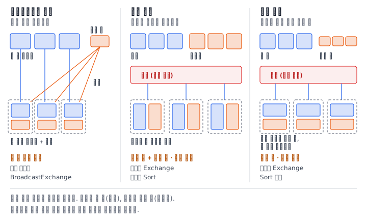
Broadcast hash join (BroadcastHashJoin). The driver collects the small-side table and sends one copy to every executor. The executors build a hash table from it, and each partition of the large side looks it up in place. There is no shuffle on the large side. So it is the fastest, but the small side has to be really small, because it is loaded whole into the memory of the driver and every executor.

The criterion by which Spark chooses this automatically is spark.sql.autoBroadcastJoinThreshold in the performance tuning documentation. The default is 10MB, and if the table size seen from statistics is smaller than this, it broadcasts. Setting it to -1 turns automatic broadcast off. spark.sql.broadcastTimeout in the same documentation is the time to wait for the broadcast, 300 seconds by default.

Sort merge join (SortMergeJoin). It shuffles both sides by the hash of the join key so that the same key gathers in the partition with the same number. Then in each partition it sorts both sides by key and scans the two lines side by side to match pairs. Both sides pay the shuffle and sort cost, but the sort can spill to disk when memory runs short, so it gets to the end at any size. That is why this is the default choice when both tables are large.

Shuffle hash join (ShuffledHashJoin). The shuffle is the same as in the sort merge. The difference is that instead of sorting, it builds a hash table from the smaller side for each partition. It can be fast because it skips the sort, but the smaller side of one partition has to fit in memory. So Spark chooses this only when the conditions are met.

from pyspark.sql import functions as F

orders.join(products, "product_id").explain()            # 작으면 BroadcastHashJoin
orders.join(F.broadcast(products), "product_id")         # 크기와 상관없이 브로드캐스트
orders.join(products.hint("shuffle_hash"), "product_id") # ShuffledHashJoin 요청
orders.join(products.hint("merge"), "product_id")        # SortMergeJoin 요청

When reading a plan, look not at the name of the join but at what is attached beneath it. For a sort merge, each branch on both sides gets one Exchange hashpartitioning(product_id, …) and one Sort: two shuffles and two sorts. For a broadcast, only the small side gets a BroadcastExchange, and the large side's branch has no Exchange. For a shuffle hash, there is an Exchange on both sides but no Sort. If you get used to these three shapes, you can see what was moved without looking for the join name.

Hints and their limits

Sometimes the estimate is wrong. A source without statistics such as a CSV, or a result that has passed through several filters, is hard to size. In that case, a hint is how a person tells Spark the strategy. The join hints that the hints documentation lists are four: BROADCAST (aliases BROADCASTJOIN and MAPJOIN), MERGE (aliases SHUFFLE_MERGE and MERGEJOIN), SHUFFLE_HASH and SHUFFLE_REPLICATE_NL. The side with a BROADCAST hint is broadcast regardless of the threshold. In the DataFrame API, the broadcast() function does the same thing.

If you attach different hints to the two sides, the earlier one wins in the order BROADCAST, MERGE, SHUFFLE_HASH, SHUFFLE_REPLICATE_NL. And the performance tuning documentation states clearly: a hint is not a guarantee. This is because some strategies do not support certain join types. For example, in a left outer join, all rows of the left side must be kept, so the left side cannot be broadcast and used as a hash table. So after adding a hint, always check in the plan what was actually chosen.

A plan that changes during execution: AQE

Adaptive query execution (AQE) has been on by default since 3.2.0. After a shuffle has finished, AQE looks at how many bytes actually came out and rewrites the rest of the plan. What matters for joins is the rule that changes a sort merge into a broadcast hash. According to the performance tuning documentation, it changes when one side, as seen by the runtime statistics, is smaller than the adaptive threshold (spark.sql.adaptive.autoBroadcastJoinThreshold, which by default is the same as the automatic threshold).

The documentation attaches an honest caveat here. It is not as efficient as planning a broadcast from the start, because the shuffle has already happened. In exchange, it avoids sorting both sides, and if the local shuffle read is on, it reads the shuffle files in place without the network. In the plan, you can see that what was AdaptiveSparkPlan isFinalPlan=false at first becomes isFinalPlan=true after execution, and that the join name has changed inside it.

There is also a rule that changes a sort merge into a shuffle hash. It changes when all partitions after the shuffle are smaller than spark.sql.adaptive.maxShuffledHashJoinLocalMapThreshold, but the default of this value is 0, so it does not happen unless you turn it on separately.

What it looks like in the field

First, the number of rows grows after a join. If the join key is not unique on one side, the pairs multiply. If an order has three rows of the same product in the promotion table, that order becomes three rows. The revenue total looks inflated and the report is wrong, yet not a single error appears. The habit of counting the uniqueness of the small side's key before joining prevents this accident.

Second, a broadcast kills the driver. If you raise the threshold a lot or overuse hints, a table of several hundred MB is collected on the driver and then copied to every executor. Driver out-of-memory or broadcast timeouts occur at this point.

Third, when looking for "what is missing", use an anti join instead of filtering nulls after an outer join. The join documentation defines an anti join as a join that returns the rows of the left side that have no match on the right. The question of finding customers who have never placed an order is exactly this shape, and only the left columns remain in the result.

What really matters in practice

• The join strategy is a choice of what to move. If you copy the small side, the large side does not move.
• The criterion for automatic broadcast is 10MB. For a source without statistics, the estimate can be wrong.
• A hint is a request, not a command. After adding one, check the actual name in the plan.
• AQE changes a sort merge into a broadcast during execution. But the shuffle already paid for is not refunded.
• Count the uniqueness of the key before joining. A duplicated key inflates rows without an error.

What you will do in the next lab

You join the orders with the small products table and confirm from the plan that Spark chooses a broadcast by itself. You turn off the threshold to see it change to a sort merge, and change the strategy directly with the broadcast and shuffle_hash hints. With the threshold left low, you catch in the final plan the moment AQE changes a sort merge into a broadcast during execution, count how the duplicated keys of the promotion table inflate rows by comparing with the row count of a left_semi join, and then find the customers with no orders with an anti join.